Lab 2: Capturing Signals, and Displaying Signals in Matlab
Overview
Last week you used an integrated program, gqrx or SDR#, to control your SDR and listen to sideband commercial FM, and narrowband FM used in police and fire radio. This week we'll get a little closer to the hardware, and learn how to control the SDR's more directly. We'll use this to save data to a file, or stream it over a socket, so that we can get signals into matlab where we can get a better look at them.
Aims of the Lab
This week we'll look at other ways to control your SDR, how to get the data into matlab, and then display the spectrum. In the end you will be able to capture a signal, and display it's spectrum as a plot, and a spectrogram which displays how the spectrum changes with time.
Command Line SDR Control
You can control your SDR more directly with programs you run from the command line. This will allow you to see details about the SDR, capture data to a file, or stream it over the network via a socket.
If you have a mac, the programs used to be installed when you installed gqrx. However the latest version does't. The easiest thing to do is install an older version that includes these. This is at
Just make sure to give it a unique name so you don't write over the latest version of gqrx.
They are stored in the directory that is the application. Open a terminal, and cd to
/Applications/Gqrx_2.11.5.app/Contents/MacOS/.
Here I assume you named the old version Gqrx_2.11.5. This has several programs, including three that you will be using in this lab. These are rtl_test, rtl_sdr, and rtl_tcp.
Either add the directory where these programs reside to your path, or make symbolic links to them, so that you can run them conveniently.
You can also build these using Homebrew or Macports.
If you are using Windows you can download and install the executables directly from Osmocom, the company that supports all of these projects. The link to the general page is
and a link to the compiled binaries is
Executables for the rtlsdr utilities
Choose the latest version compatible with your system.
For Linux you can install gqrx using the apt manager, and this will automatically install all of gnuradio and the rtl utilities.
rtl_test
The first program we'll look at is rtl_test. This looks for the SDR, and reports what it finds. This is the first program use when debugging your SDR.
> rtl_test
Found 1 device(s):
  0:  ezcap USB 2.0 DVB-T/DAB/FM dongle

Using device 0: ezcap USB 2.0 DVB-T/DAB/FM dongle
Found Rafael Micro R820T tuner
Supported gain values (29): 0.0 0.9 1.4 2.7 3.7 7.7 8.7 12.5 14.4 15.7
16.6 19.7 20.7 22.9 25.4 28.0 29.7 32.8 33.8 36.4 37.2 38.6 40.2 42.1
43.4 43.9 44.5 48.0 49.6

Info: This tool will continuously read from the device, and report if
samples get lost. If you observe no further output, everything is fine.

Reading samples in async mode...
^CSignal caught, exiting!

User cancel, exiting...
This runs continuously to test the data rate, until you stop it with a ^C. There are a number of options, which you can see with the “-h” command line option (which isn't actually an option).
> rtl_test: illegal option -- h
rtl_test, a benchmark tool for RTL2832 based DVB-T receivers

Usage:
	[-s samplerate (default: 2048000 Hz)]
	[-d device_index (default: 0)]
	[-t enable Elonics E4000 tuner benchmark]
	[-p enable PPM error measurement]
	[-b output_block_size (default: 16 * 16384)]
	[-S force sync output (default: async)]
You can set the sampling rate with the “-s” option, which defaults to 2.048 MHz. One interesting option is “-p”, which tests what the actual sampling rate is. This will be slightly off of what you've asked for, and is the reason that the peaks in the spectra aren't exactly where they should be when you use gqrx or SDR#. This changes as the device heats up. This is what I get after about a minute or so
> rtl_test -p
Found 1 device(s):
  0:  ezcap USB 2.0 DVB-T/DAB/FM dongle

Using device 0: ezcap USB 2.0 DVB-T/DAB/FM dongle
Found Rafael Micro R820T tuner
Supported gain values (29): 0.0 0.9 1.4 2.7 3.7 7.7 8.7 12.5 14.4 15.7
16.6 19.7 20.7 22.9 25.4 28.0 29.7 32.8 33.8 36.4 37.2 38.6 40.2 42.1
43.4 43.9 44.5 48.0 49.6
Reporting PPM error measurement every 10 seconds...
Press ^C after a few minutes.
Reading samples in async mode...
real sample rate: 2047990
real sample rate: 2047837
real sample rate: 2047994
real sample rate: 2047987
real sample rate: 2047892
real sample rate: 2047993
^CSignal caught, exiting!

User cancel, exiting...
Cumulative PPM error: -27
This shows that my sampling rate is off by -27 parts per million, or ppm. You can set a correction for this in gqrx or SDR#.
rtl_sdr
The next program is rtl_sdr. This starts the SDR up, and then collects data and writes it to a file. This also has a number of options
> rtl_sdr
rtl_sdr, an I/Q recorder for RTL2832 based DVB-T receivers

Usage:	 -f frequency_to_tune_to [Hz]
	[-s samplerate (default: 2048000 Hz)]
	[-d device_index (default: 0)]
	[-g gain (default: 0 for auto)]
	[-b output_block_size (default: 16 * 16384)]
	[-n number of samples to read (default: 0, infinite)]
	[-S force sync output (default: async)]
	filename (a '-' dumps samples to stdout)
You set the center frequency with the “-f” switch, specified in Hz (you will get a lot of practice counting zeros!). The “-g” switch sets the gain in dB. You can set it to anything, but you'll get the closest value from the list of supported gains that you saw with rtl_test. For example to collect 10 seconds of data centered at 120 MHz (the AM air band used for air traffic control), you would run
> ./rtl_sdr -f 120000000 -g 40 -n 20480000 ab120_10s.dat
Found 1 device(s):
  0:  Realtek, RTL2838UHIDIR, SN: 00000001

Using device 0: ezcap USB 2.0 DVB-T/DAB/FM dongle
Found Rafael Micro R820T tuner
Tuned to 120000000 Hz.
Tuner gain set to 40.000000 dB.
Reading samples in async mode...

User cancel, exiting...
The program terminates by itself when it has collected enough data.
Once we've saved the data to a file, we can load it into matlab. This m-file does the this
which looks like this:
function y = loadFile(filename)
%  y = loadFile(filename)
%
% reads  complex samples from the rtlsdr file
%

fid = fopen(filename,'rb');
y = fread(fid,'uint8=>double');

y = y-127;
y = y(1:2:end) + i*y(2:2:end);
This loads the signed sequence of byte I and Q values, and stores them as complex matlab vector.
Airband AM Signals
The main part of the lab is to capture and decode AM signals in the air band, with is right above the commercial FM band we were decoding last week. There is a band from 108-118 MHz that mostly has navigation beacons that identify themselves by Morse code. Then from 118-137 MHz there are several bands used for communication between aircraft and the ground. Communications in these bands uses AM modulation. This is because when two users try to talk on the same channel, you hear both of them with AM. With FM, you hear only the stronger of the two, or something completely intelligible if both are the same strength. With air traffic control, it is important to hear everyone that is out there!
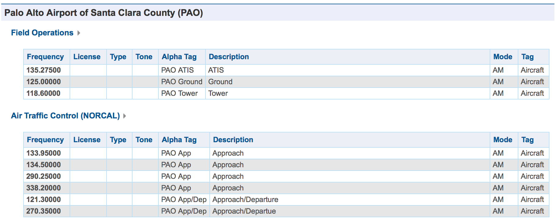
The local airport is Palo Alto, which is station KPAO. It transmits on these frequencies
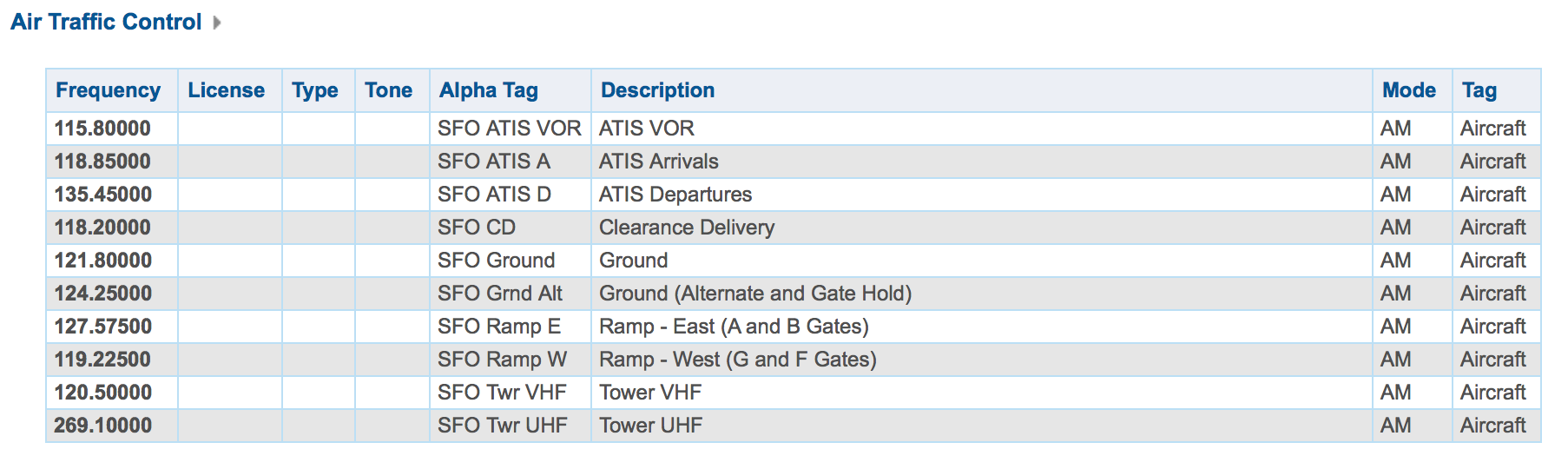
We will also hear traffic from San Francisco (SFO), San Jose (SJC), as well as NORCAL Approach, which coordinates the airspace. The frequencies for SFO are
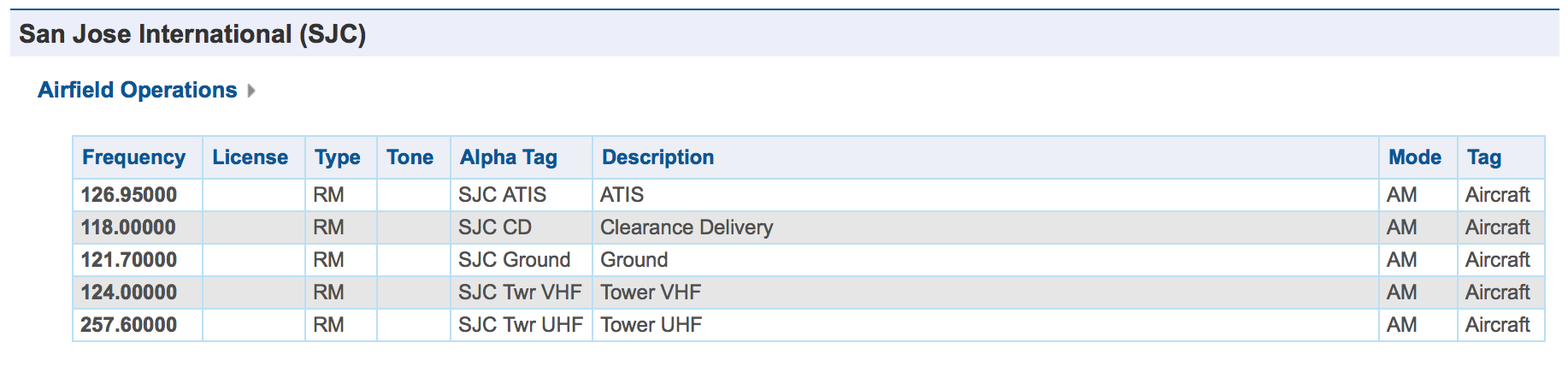
and San Jose are
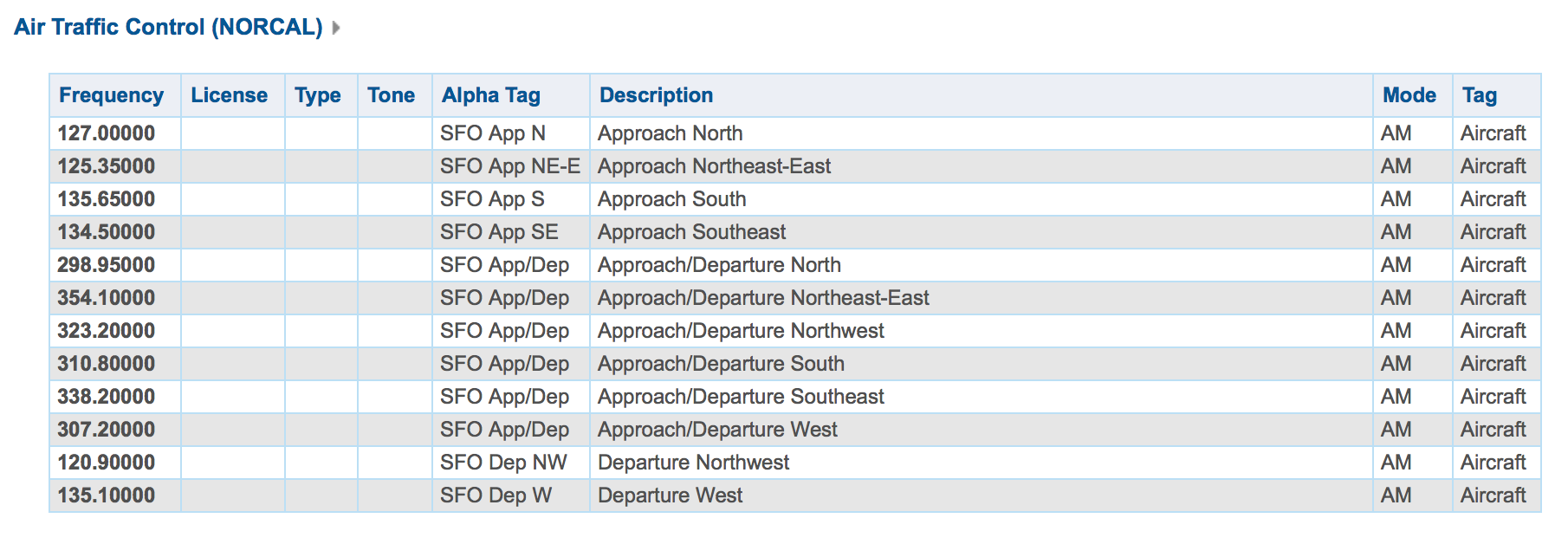
and Norcal Approach are
Choose a frequency where you might expect to get a signal. The ATIS frequencies are good initial candidates, because these continuously transmit information about the airport, and how to contact them. The other frequencies, such at the air traffic control frequencies, are more interesting, but are not always in use. Often a transmission lasts just a few seconds, and can be hard to capture.
One busy channel that has a strong signal around here is 310.8 MHz, SFO departures and arrivals from the south. This frequency also is a good match for your SDR antenna. At 310.8 MHz a quarter wave antenna is 24 cm, or about 9.5 inches. Stick your antenna to a metal surface to provide a ground plane, and extend the antenna to this length. Small adjustments to the frequency can help (+/- a few kHz).
Use gqrx or SDR# to see if you can find any activity. Here is an example
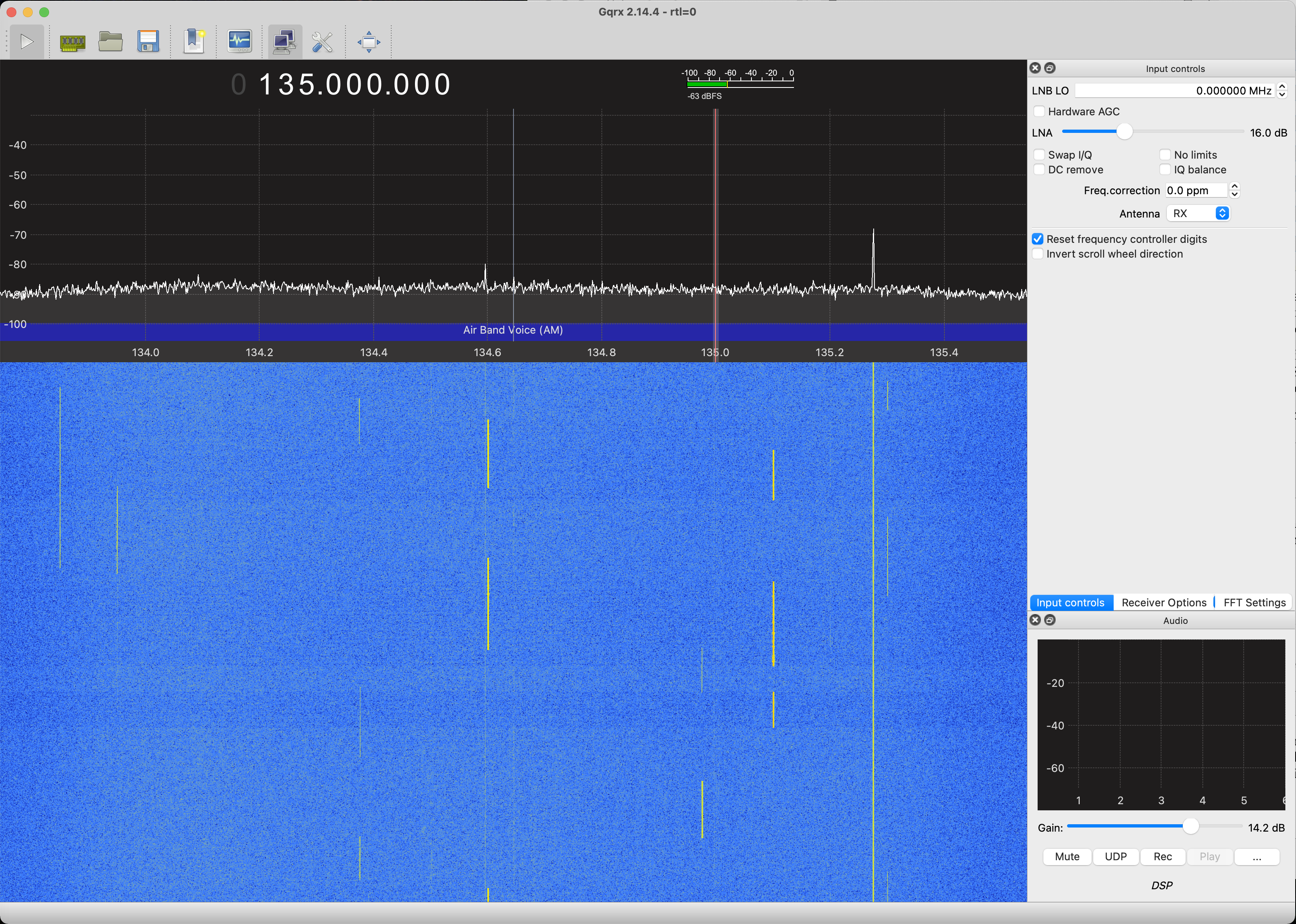
You see a couple of frequencies in use. The one that is on continuously is an ATIS signal. The others are planes and towers talking to each other. Note the gain you use here, so you can set it to be the same for your capture.
Once you know there is a signal out there, capture 10 seconds of data, and save it to a file. Close gqrx or SDR# to free up the SDR, and then capture the data with
> rtl_sdr -f 135000000 -n 20480000 ab.dat
where I have chosen 135.0 MHz. You will probably want to set it to something else. Don't set the frequency exactly to the frequency you want to acquire, because the receiver produces an artifact at DC. This is the spike you always see at the middle of the spectrum.
A sample file is available at
You can use this file if you are having trouble finding signals to capture. It is sampled at 2.048 MHz, and is centered at 135.5 MHz. The Palo Alto ATIS signal is there, as well as one of the NORCAL approach signals
Once you have the data, we will load it into matlab to look at it. Start up matlab, and change to the directory where loadFile.m and the data file are. Load the data file with
>> d = loadFile('ab.dat')
The first thing to note is that just 10 seconds of RF is a lot of data! It is hard to tell if we have anything, or how to extract it. What we will do is make something like the waterfall plot that you see in gqrx or SDR#, called a spectrogram. What this does is compute the spectrum of blocks of the signal, and displays an image of how this changes over time. A basic spectrogram program is provided here
It is msg.m for “my spectrogram”. We will improve this as the course goes on. The help information is
>> help msg

  msg(x,n0,nf,nt,dbf)

   Computes and displays a spectrogram

       x  -- input signal
       n0 -- first sample
       nf -- block size for transform
       nt -- number of time steps (blocks)
       dbf -- dynamic range in dB (default 40)

   This extracts a segment of x starting at n0, of length nf*nt
   The image plot is in dB, and autoscaled.  This can look very noisy
   if there aren't any interesting signals present.
This takes an input signal starting at sample n0, and computes the spectrum of nt segments of the signal, each of length nf. The result is displayed as an image, with time going horizontally, and frequency vertically. The center frequency is in the middle of the plot. For example, for the data provided above, we can look at the first second of data, by looking at 2000 blocks each of length 1024 samples (2048000 total samples, or one second at the 2.048 sampling rate). The results is
>> d = loadFile('ab1335_10s.dat');
>> msg(d,1,1024,2000);
Unless you have a very big display, you'll get an error message that the image doesn't fit, and was scaled down. The result looks like this
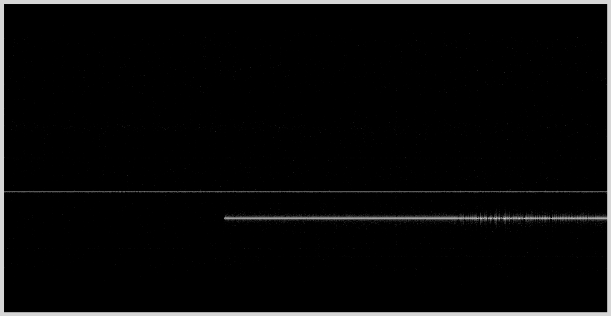
We see several signals. The msg.m file will return the data that is plotted if you assign the output to a variable
>> ds = msg(d,1,1024,2000);
We can plot the spectrum at at time of 0.5 seconds by plotting column 1000,
>> plot(abs(ds(:,1000));
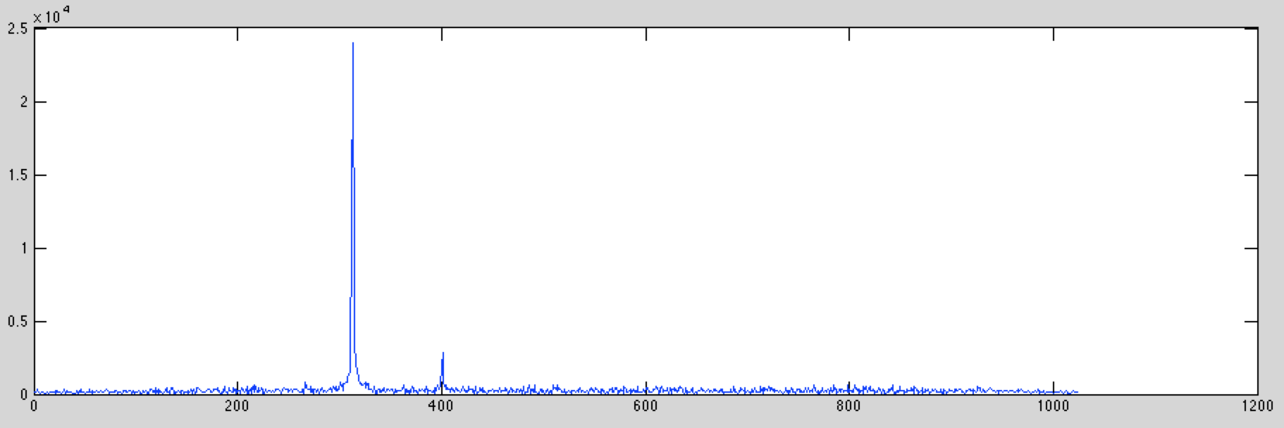
By zooming in, you can see that there is a strong signal at sample 313. You can plot that signal by plotting a row of the data
>> plot(abs(ds(313,:));
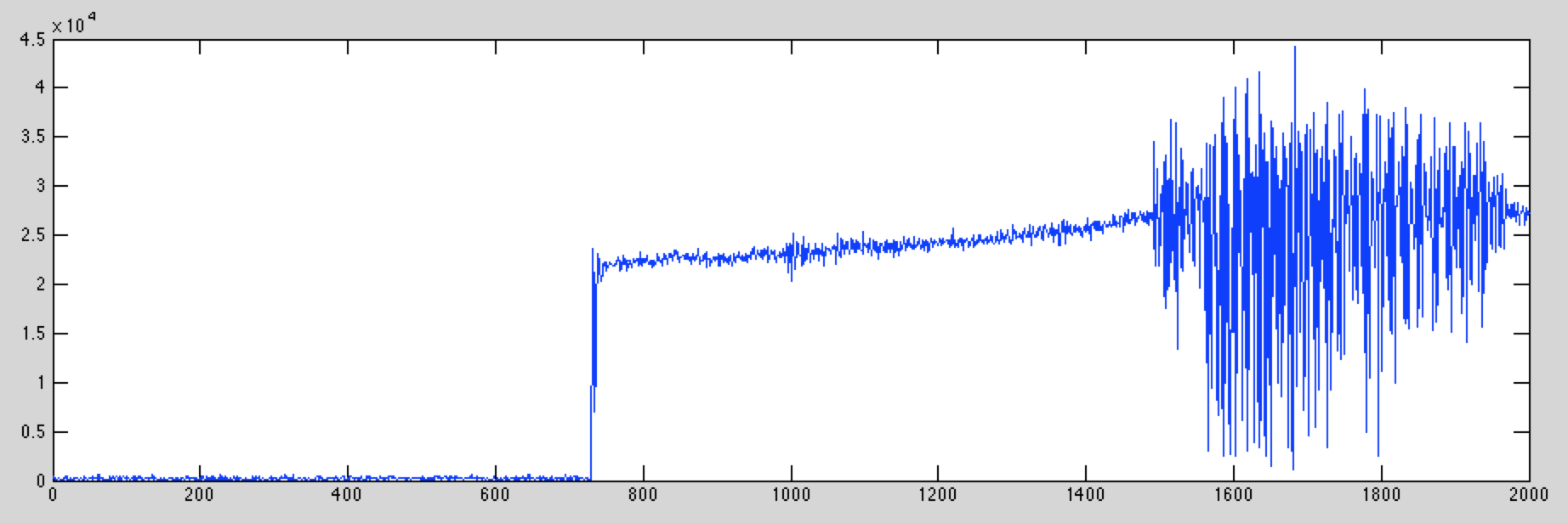
What you see is a conventional AM signal. The transmitted signal is a constant bias plus the voice signal being transmitted.
For your assignment, find an AM signal in the data you captured, and email me a screen shot of a plot of the signal. Or, if you are using the data set provided, find another signal, and send a plot of it (there are at least two more). You have ten seconds of data, so you can look later in the signal by increasing n0. For example, to start at 5 seconds, n0 should be 5*2048000.
You can also use msg.m to decode the signals. Each column in the image is a sample of the spectrum in time. If we want to sample at 8kHz, we need blocks that are 2048000/8000 = 256 samples. In this case the entire data set is 80,000 samples. You may want to comment out the imshow line, and then do
>> dd = msg(d,1,256,80000);
Find the row in dd that corresponds to your signal, take the absolute value, scale it to a maximum amplitude of one, and then play it through your sound card. You should hear the audio.
>> dx = abs(dd(N,:))
>> dx = dx/max(dx);
>> sound(dx,8000);
Next time we'll look at better ways to do this using modulation and decimation.